Practical Finite Element Analysis, ABAQUS Python Scripting: My Course on Udemy

Right now, there are more than 5000+ job advertisements, globally, for keywords “Finite Element Analysis (FEA)” and “Computer Aided Engineering (CAE)”. The pay for these jobs are spiking up and the demand too is increasing at an insane rate. 

The reason is simple. Almost all companies have realized the importance of simulation-assisted design processes. They are figuring out ways to incorporate simulation in their product development lifecycle and need skilled people who can help them do that.

But here’s the catch.

Companies want people who understand the bigger picture of things and adapt to the ever-changing landscape of product design. Not someone who knows the theory but finds it difficult to apply it in real life.

This course is exactly intended to bridge that gap between FEM theory and application

https://www.udemy.com/course/practical-finite-element-analysis-abaqus-python-scripting/?referralCode=280EF78F68173642922D

I will take you through different steps in Finite Element Analysis from a practical perspective. It is going to be fully application-oriented and I will present some case studies from the industry that will give you an idea of how industry professionals break down complicated problems into small chunks and then solve them gradually. I will also talk about the physical meaning of a lot of commonly misunderstood terms and terminologies in FEA. It’s always teamwork going ahead and these terminologies would help you to communicate effectively with other FE Analysts and design engineers in your team.

Then, I will introduce a framework for Python scripting that could be used for simulating problems with ABAQUS. I will use this framework to help you write Python scripts for 4 different problems and solve it using ABAQUS.

Let me go ahead and reveal a secret. If you are not going to be a FEM tool developer, you don’t need all the math that is being taught at the university or being described in detail in standard FEM textbooks. Rather, you need a clear and conceptual understanding of the concepts of FEA and then the aptitude to select and use the right tools from the commercially available FEA packages. 

That will be this course’s contribution to you.

Towards the end of the course, I will also reveal some tips to prepare your career for landing a job as a FE Analyst.

What are you waiting for? Act now and get yourself certified with this course.

https://www.udemy.com/course/practical-finite-element-analysis-abaqus-python-scripting/?referralCode=280EF78F68173642922D

Who is this course for?

• Mechanical / Civil Engineering students who want to understand FEA in a practical way without getting bombarded with complicated math
• Beginner FE Analysts from the industry who want to apply FEA right away in their work routine
• Design engineers looking to transition into a FE Analyst role
• Engineers who want a framework for using Python Scripting in ABAQUS to increase productivity
• Managers who want to understand the bigger picture of FEA before decision making
• Technical Sales Professionals who want to be sure about the fundamentals of important terms used in FEA
• Small or medium sized companies who are short on manpower and time and who want to quickly ramp up their understanding of FEA 

https://www.udemy.com/course/practical-finite-element-analysis-abaqus-python-scripting/?referralCode=280EF78F68173642922D

What you’ll learn?

• Understand the fundamentals of Finite Element Analysis (FEA) from a practical perspective without complicated math or equations
• Top-down and Bottom-up approach in FEA
• Steps in a FE Analysis and Examples of FE Applications
• Assumptions, Advantages and Limitations of FEA
• Types of FE Analysis: Static, Dynamic, Modal, Fatigue, Thermal, Heat transfer
• Using Symmetry, Plane Strain and Plane Strain conditions
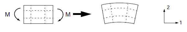
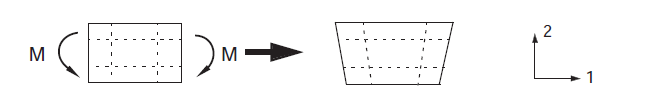
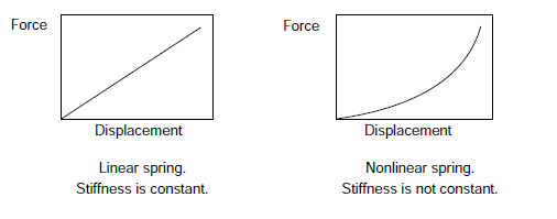
• What is Geometric-nonlinearity and when to use it
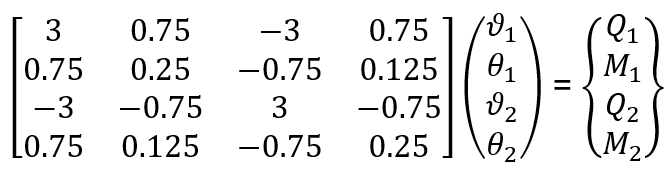
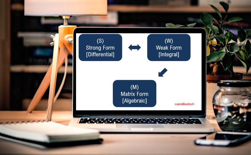
• Difference between strong forms and weak forms in FEA
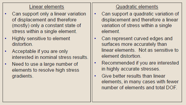
• Types of elements and coordinate systems
• Difference between Plate, Shell and Membrane Elements
• Meshing: Quality check and Convergence
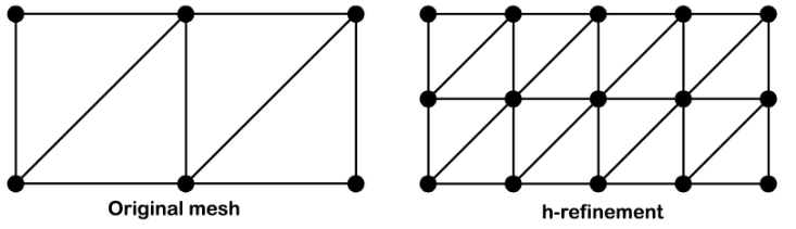
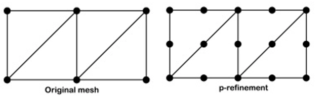
• Difference between h and p method
• Physical meaning of full and reduced integration
• What do shear locking and hourglassing mean in a practical context?
• Difference between essential and natural boundary conditions
• Direct and Iterative solvers: What’s the difference?
• Verification and validation in simulation
• Error Sources in FEM
• Industrial Case Study: Static Characteristics of a milling machine
• Industrial Case Study: FE Analysis of a slewing bearing of a wind turbine
• 6 things to consider before starting any FEA and a generic problem solving methodology
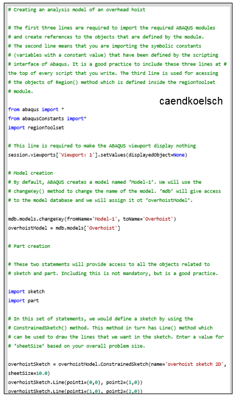
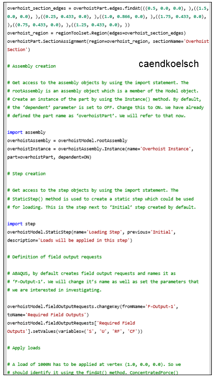
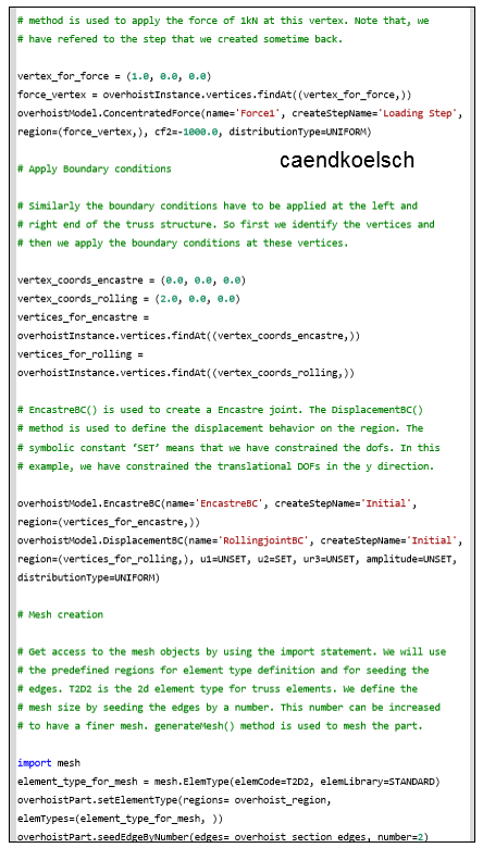
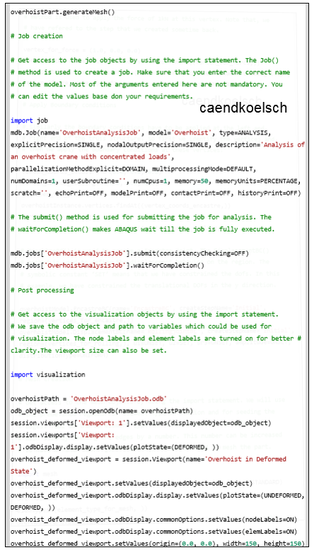
• Introduction to Python Scripting in ABAQUS and a general workflow for running a Python Script in ABAQUS
• A higher level understanding of Python Scripting methodology for ABAQUS
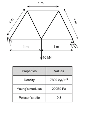
• Example 1: Python Scripting of a static analysis of a truss
• Example 2: Python Scripting of a deflection analysis of a cantilever beam
• Example 3: Python Scripting of a steady state thermal analysis
• Example 4: Python Scripting of a truss parameterization problem
• FEA in 2021: What to expect
• Communicate effectively with all stakeholders of a product design process
• How to mold your thought process as a student to get a job in FEA
• Understand how to accumulate that “experience” that big companies want before they hire you
• How to get an insider perspective and get hired as a FE Analyst

https://www.udemy.com/course/practical-finite-element-analysis-abaqus-python-scripting/?referralCode=280EF78F68173642922D

Requirements

• Basic knowledge of Mechanical / Civil engineering. There will be no math in this course
• Any text editor. I use Notepad++ because it’s free and doesn’t occupy much space. You can choose your own text editor 
• Student version of ABAQUS is sufficient

https://www.udemy.com/course/practical-finite-element-analysis-abaqus-python-scripting/?referralCode=280EF78F68173642922D

Some tips for beginners and FEM enthusiasts (Links to Learning Resources)

Hello folks,

This is the place where I would consolidate all the open-source material on tips and techniques relevant to FEA. I hope to update this list continually.

Happy Learning.

=============================

Post Processing:

Performing an FE analysis is one thing. Understanding the results, interpreting and documenting them is another task that is of equal importance. I recently found this link from Altair University on Post-processing. It’s my opinion that our textbooks or university courses do not emphasize much on the post-processing part. This is also partly due to the fact that this topic is software specific.

But there are some common aspects which need to be known if you wish to become an expert in FEA. These common aspects are greatly captured in the link below.

https://altairuniversity.com/wp-content/uploads/2012/04/Student_Guide_307-342.pdf

I thoroughly enjoyed reading this link and picked up some basic things which I ought to have known before. In case you haven’t read this before, please do consider reading it once. Worth your time.

=============================

How to get meaningful and correct results from your finite element model?

I recently read this and found it to be really informative. Go through the detailed list and take notes if necessary.

https://arxiv.org/pdf/1811.05753.pdf

=============================

General FEA related blogs (Worth your time)

Best & extremely practical – https://enterfea.com/blog/

And of course mine (Ha ha)

=============================

Regards,

Renga

ABAQUS Python script for carrying out a static analysis of an overhead hoist & some tips for naming variables in a script

Writing Python scripts for ABAQUS drastically increases your productivity as a CAE analyst. You can automate a lot of repetitive tasks as well as avoid trivial errors that amateurs make.

If you have already started/tried Python scripting for ABAQUS, you would have noticed the scarcity of step by step tutorial documents or guidelines. But this should not stop you from becoming an expert in Python scripting which is actually easy if you start with the right mind and resources.

Through this post, I would like to carry out static analysis of an overhead hoist using Python scripting in ABAQUS and thereby highlight its usefulness. Similar to other pursuits in general, Python scripting for ABAQUS looks difficult at the beginning. But once you have a clear understanding of the workflow and are able to identify a pattern in problem solving, it is just a matter of time and practice before you become skilled in it.

Note: This article is the second chapter from my book

Crash Course on Python Scripting for ABAQUS: Learn to write python scripts for ABAQUS in 10 days

Okay, let’s get started with the example.

We are interested in finding the static deflection of an overhead hoist structure. The structure is a truss which is constrained at the left end and mounted on rollers at the right end.

The example is taken from the ABAQUS user manual. Figure 1 shows the schematic of the overhead hoist. All members are circular steel rods, 5 mm in diameter.

Figure 1 Schematic of the overhead hoist  (DS Simulia, 2008)

A 10 kN load is applied on one of the nodes and the static deflection of the truss structure needs to be estimated. Once we will write the script for this task, we can use the same script for finding the dynamic response by making slight modifications (Refer my book for this example – You can also write this on your own after you understand this script).

Let’s get started.

Python script:

For solving this problem, you will have to

• Sketch the truss
• Define the material
• Create a section and assign it
• Create an instance and step
• Define the boundary conditions and loads
• Mesh the part
• Create the job, submit it and carry out post-processing

You would have to perform the above steps for every analysis that you wish to do in ABAQUS. Having this work sequence in mind can help you write the script more efficiently.

‘One main word’ strategy:

In all the scripts that I write, I will be using an idea, which I would like to call as ‘One main word’ strategy. I will choose this ‘One main word’ based on the problem context and use it while naming the variables. You will appreciate this strategy as it will eliminate the need to keep thinking new variable names as well as avoid silly mistakes in the process.

For example, this example deals with an over hoist structure. So, I would be naming variables in the likes of overhoistModel, overhoistPart, overhoistSection, overhoistMaterial, etc.,

As you can see, ‘overhoist’ is the one main word which I will be using throughout. You will understand this much better as you read the script. I have added comments into the code wherever required.

Comments are statements that begin with #. These comments contain all the information as well as the explanation you need for writing these Python scripts.

Summary:

Do not worry if  you don’t understand each and every line in the script. It is totally natural at this point of learning to write Python scripts for ABAQUS. Do not panic!

As of now, try to mentally connect the input arguments that we used  for the methods in the script with the ones that we define when we use the ABAQUS CAE Graphical User Interface(GUI).

With constant practice, I am sure, you would get a clear picture of the scripting practice and would start writing scripts on your own.

You can also copy and paste some parts of this script directly into your script and just make minor modifications. For example, from the material definition or from the Post processing section. This will save you a lot of time if you have to repeatedly use the same material for a number of simulations or would like to generate similar output reports every time after you complete a simulation.

To summarize, in this article we learnt how to write a Python script for finding out the static response of an overhead  hoist with a point load of 1kN. The script can also create a view port for visualization of the simulated results after successful completion of the job.

All the best for an effective learning. Before I conclude this article, I want to list out 4 tips for naming variables in your script.

Tips for naming variables while writing Python scripts for ABAQUS

If proper variable names are used, it improves the readability, re-usability of your code and helps in extending the scope of the code as well.

These rules also cover most of the mistakes that beginners usually make. So stay aware of them!

Rule 1:

A variable name cannot start with a number. It can start with letters and then have numbers and underscores.

Correct:  vertices_for_force  Incorrect: 1vertex

Rule 2:

Avoid the usage of python keywords like raise, class, def, with, yield, lambda, etc.,

Rule 3:

Spaces are not allowed in a variable name. Use an underscore if you have two words in a variable name.

Correct:  vertices_for_force  Incorrect: vertices for force

Rule 4:

Variables must be descriptive of what they represent. Avoid the usage of variable names with a single alphabet though it might be easy initially.

Hope this helps. Have a great day.

Prost!

~ Renga

If you like this post, I am sure you would be liking my book as well.

Many people who bought the book have either emailed me or registered their opinions on the Amazon page stating that they have found the book to be useful.

You are just a click away from becoming a skilled person in ABAQUS Python scripting.

Crash Course on Python Scripting for ABAQUS: Learn to write python scripts for ABAQUS in 10 days

Go ahead and buy the book. I am sure, you will never regret it.

A note about the reviews:

Strangely, Amazon.com only shows the reviews made by buyers from the USA. There are great reviews published on the German, Canadian and the Indian version of Amazon as well. Unfortunately, I am not able to link the reviews from these country websites in to the USA version. If you want to know what people all over the globe are thinking about the book, please visit the respective country websites.

Difference between h-method and p-method in FE Analysis (FEA)

There are basically two discretization approaches in FE analysis which are used to increase the solution accuracy as well as check for numerical convergence.

1. h-method

In this method, the number of elements is increased to have a finer mesh. The element type is not changed but only the number of the elements used for the analysis domain is increased.

“h” usually denotes the characteristic length of elements. This method is about reducing the “h” value which results in increased number of elements.

Figure 1: h-method [1]

If we look at the stress contours of a geometry which is approximated by a very coarse mesh (reduced number of elements), the stress distribution might deviate very much from the actual results and sometimes might also have stress jumps. This calls for a finer mesh as seen in the above picture.

2. p-method

This is the other method to increase the numerical convergence and move towards a more accurate solution. Here, the order of the shape functions is increased instead of increasing the number of elements. “p” denotes the polynomial order. By default, linear order shape functions are used by commercial FE programs. A quadratic shape function can have more accurate solutions.

Figure 2: p-method [1]

About the usage of p-element method from Altair University’s “Practical Finite Element Analysis” book

It has been documented in this book that the p-method is usually recommended for design engineers (CAD) who are in the initial design phase. At this point of the product design life cycle, they would not be too worried about carrying out a detailed analysis. Once the design engineers are satisfied with a basic feasibility analysis, they transfer the CAD data to the CAE team who in turn carry out the detailed and in-depth analysis.

So it is a god assumption to think in the lines of the p-method being used by the design (CAD) team in the initial phase and then the h-method being used by the analysis (CAE) team where detailed investigations and analysis need to be carried out.

And below is a snapshot [2] which complements the current discussion topic.

Prost!

~ Renga (Renganathan Sekar)

References:

[1] https://deust.wordpress.com/2014/11/30/h-method-p-method/

[2] http://innomet.ttu.ee/martin/MER0070/Loengud/FEA_Best_Practices.pdf

 

A book on Python Scripting for ABAQUS:

I have written a book that helps you to write Python scripts for ABAQUS in just 10 days.

Why should you buy my book?

Please use the link below to purchase the book.

Crash Course on Python Scripting for ABAQUS: Learn to write python scripts for ABAQUS in 10 days

Direct vs. iterative solvers in FEM

In FEM we usually solve for the equation [K]{u} = {f}

Here [K] is referred to as the stiffness matrix; {f} as the force vector and {u} as the set of unknowns.

The classification of solvers into direct and iterative mainly depends on the method of getting {u} in the linear equation. The selection of the solver depends on the process mechanics and problem size and is nowadays automatically chosen by most of the commercially available FE tools.

But as an engineer and analyst, it is good to know the back-end of what’s happening with respect to the solver selection. So here we go with a non-mathematical explanation of the differences between direct and iterative solvers used in FEM.

Direct Solver:

In the case of direct solver, you find the inverse of matrix [K] and then multiply with {f}. As this method involves inverting the matrix, it is mostly preferred for computationally less expensive problems. From literature, I understand that direct solvers are effective for problems with less than 100,000 unknowns. And the memory requirements are higher and the ability to solve the equations in parallel is difficult but not impossible.

Usually the direct solvers can be thought of as a variant of LU decomposition method where the [K] matrix is decomposed into a lower and upper triangular matrix (L and U respectively) in such a way that

[K] = [L][U]

More details about the method can be found here.

FE developers exploit the sparsity patterns in the stiffness matrix to increase the computational efficiency in the case of direct solvers by using established algorithms for solving sparse matrices.

What is a sparse matrix? – Read here.

Iterative Solver:

In the case of iterative solver, since finding inverse of a matrix is very time consuming if it is a very big matrix, they start with an initial solution(guess) and then gradually move towards the correct solution for {u}. Till a reasonably solution that satisfies the stop criterion (a tolerance value, usually) is obtained, the solver keeps iterating.

So, this is also not an exact solution but an educated guess. The search direction, i.e. the direction in which the initial guess moves towards the final solution is verified by using a variant of conjugate gradient method.

Iterative solvers are suitable for computationally big problems as they can often be parallelized more efficiently using algorithms. But there is a catch. For solving the linearized equations using the iterative solvers, your matrix needs to be properly conditioned.

“The art of devising a good iterative solver is to devise a good preconditioner!”.

–  Prof. Wolfgang Bangerth,

In the case of iterative solvers, sometimes oscillatory behavior might be observed. This means the initial solution does not move gradually towards the correct approximate solution and rather diverge. As an end user, you can find this by constantly checking the numerical output that is written by the solver. Unusually long computational times can also be a good indicator for this kind of a problem.

So how can you fix it?

Again, this method is something that has worked for me most of the time. My approach would be to check the model thoroughly if it is constrained properly. As in, try to fix the DOFs (DOF – Degree Of Freedom) in your analysis domain that might not have an impact on the simulation results. By doing this, you are reducing the potential errors gradually and assisting the solver converge fast.

And this is a very simplified and non-mathematical explanation of the topic which could be useful for a beginner or an application engineer who just wants to know which solver to use based on the problem context.

For a detailed and mathematical explanation, I would recommend going through this link. https://link.springer.com/chapter/10.1007%2F978-3-319-59038-7_5

Prost!

~ Renga

Other references:

[1] http://www.math.colostate.edu/~bangerth/videos/676/slides.34.pdf

 

A book on Python Scripting for ABAQUS:

I have written a book that helps you to write Python scripts for ABAQUS in just 10 days.

Why should you buy my book?

Please use the link below to purchase the book.

Crash Course on Python Scripting for ABAQUS: Learn to write python scripts for ABAQUS in 10 days

What is shear locking in FEM?

Sometimes, does your FE predictions of deformation end up lesser than the theoretical predictions?

Let’s see one of the main reasons why this happens – which is shear locking.

The unintentional generation of shearing deformation rather than the desired bending deformation is actually shear locking – Due to this the element becomes too stiff and the overall deflections are lesser.

This happens mainly with fully integrated linear elements subjected to bending loads.

This problem does not arise under normal or shear loads – occurs only during loads with bending.

In this post, I would like to explain the shear locking phenomenon with the help of an example from ABAQUS user manual.

If a structure is subject to pure bending moment M, the material distortion happens as shown in Figure 1.

Figure 1: Material deformation subjected to bending moment M

This of course happens in the actual material. If this is approximated by a linear element, then the edges of the curve cannot be represented. Figure 2 shows the deformation characteristics of such an element. The dotted lines are passing through the integration points.

Figure 2: Deformation of a linear element under bending

The lengths of upper and lower lines have changed indicating that they are under tensile and compressive loading respectively. But the important observation to be done here is the change in angle between horizontal and vertical lines. Before bending, it is 90°. Now this has changed. This is an indication that there exists some shear stress at these points. But theoretically, the shear stress of a material under pure bending must be zero.

Therefore, this shear stress is referred to as “spurious shear stress” and in FE literature, the usage of “spurious nodes” can also be observed frequently.

“Spurious shear stress” is induced because the curve is not represented by the element edges.

This means that the material shears instead of bending resulting in lesser deflection overall. This in turn causes the element to be stiff.

So how can this problem of shear locking be avoided?

By using higher order elements like quadratic elements which can represent the curve along the edges, the shear locking phenomenon can be avoided.

In general, it is a good practice to stay away from linear elements if there exists a bending load in your analysis.

In the next set of posts, I will write about full and reduced integration which will make the discussion in this topic more complete.

Please comment below if you have some questions on this post.

Prost!

~ Renga

A book on Python Scripting for ABAQUS:

I have written a book that helps you to write Python scripts for ABAQUS in just 10 days.

Why should you buy my book?

Please use the link below to purchase the book.

Crash Course on Python Scripting for ABAQUS: Learn to write python scripts for ABAQUS in 10 days

 

What is nonlinearity in FEM analysis? What are the different types of nonlinearities?

Almost all the applications that one tries to solve using FEM are nonlinear in nature. It is just that the FE analyst makes an engineering assumption avoiding the nonlinearity to make the computation simple. Provided, the FE predictions do not deviate much from the actual results because of this assumption.

So, what does nonlinearity mean in a FEM analysis? What are the different types?

Continue reading to know these answers.

Of course, from a perspective of structural mechanics simulations.

Generally, linear analysis means that the relationship between the applied force and the response to this force (Ex: displacement) is linear in nature. We know that this displacement can be obtained by inverting the stiffness matrix and then multiplying it with the force vectors. In other words, this means that the stiffness matrix does not change during a linear analysis.

If you want to have a quick recap of this methodology, have a look at this article

https://caendkoelsch.wordpress.com/2017/12/03/how-are-stiffness-matrices-assembled-in-fem/.

So now consider a situation where the stiffness keeps changing as the component deforms. Like for example, a forging simulation where the effective strain values at the end of simulation go up to 5.0 or even more.

This can be further emphasized by taking the example of a spring with linear and nonlinear characteristics.

As the stiffness is dependent on the displacement, which keeps changing, the initial stiffness matrix cannot be used without continually updating and inverting it during the course of the analysis. This is the reason why nonlinear analysis takes more time to solve compared to a linear FEM analysis.

Figure1: Linear and nonlinear spring characteristics (Source – Abaqus Manual)

Now let’s look into the different types of nonlinearity:

• Nonlinearity because of material behavior

This can be understood by referring to a stress strain curve (Figure 2). After point A in the curve, the stress versus strain relationship of the material is nonlinear. This is one sort of material nonlinearity based on the deformation or strain.

Now take the case of a hot forging process. Here the deformation is also dependent on other factors, for instance – temperature.

So this summarizes the first category of nonlinearity based on the material characteristics.

Figure 2: Stress strain curve

• Nonlinearity because of geometric conditions

Geometric nonlinearity arises when the changes in the model’s geometry are very high during the course of deformation. This happens when there are

1. Large deformations
2. Large rotations
3. Both
4. Initial loading conditions before the start of the analysis

• Nonlinearity because of boundary conditions

This situation arises when there is a change in the boundary conditions during the analysis. For example, consider the cantilever beam shown below. As the vertical deflection near the end of the beam increases and hits the stop, there is a change in the boundary condition.

All other contact problems fall under this category.

Figure3: Example for boundary conditions that change during the analysis (Source – Abaqus Manual)

I will end this article with some slides from the internet that I found useful regarding contact problems

Have a good day.

Prost!

~ Renga

Source: www2.mae.ufl.edu/nkim/INFEM/Chap5.pptx

A book on Python Scripting for ABAQUS:

I have written a book that helps you to write Python scripts for ABAQUS in just 10 days.

Why should you buy my book?

Please use the link below to purchase the book.

Crash Course on Python Scripting for ABAQUS: Learn to write python scripts for ABAQUS in 10 days

What is mass scaling in simple terms?

One of the methods used in the industry to reduce the run time of an explicit FEM analysis is a technique called “Mass scaling”.

In this post, I would like to write about the physical meaning of mass scaling. Like my other posts, I will try to avoid complex mathematical equations and explain the basics. For a deeper mathematical understanding, you are advised to refer standard FEM textbooks. You can also look into the user manuals of commercial FE software like ABAQUS etc., to know how this is being implemented.

Okay, now let’s get into the topic.

The run time of a FE simulation is mainly a function of the model size (the number of degrees of freedom) and the size of the solution step.

And bigger the time step, faster the simulation. I am not talking about the accuracy here.

I just want to emphasize that the time step size has a significant impact on the run time. As the size of the model is mostly not under our control, we have to play with “Time step” to reduce the runtime.

In other words, we have to increase the time step size.

How we do this is effectively Mass Scaling.

Keep reading further.

As per the CFL (Courant-Friedrichs-Levy) condition, the stable time step for explicit analysis is

Here e_min is the size of the smallest mesh element.

c is the speed of the stress wave

The scaling factor is used for providing numerical stability.

The smallest element in the mesh has the biggest impact on the run time.

Let’s see what ‘c’ is made of.

If we increase the density of the smallest element (add mass actually!), the time step size increases which is what we want.

And you have learnt the technique of mass scaling in a very simple rhetoric.

In other words, some amount of mass is added locally near the smallest elements in the mesh, which increases the density, thereby increasing the stable time step size henceforth reducing the solution run time.

But here is the catch!

How and where to add the mass is very crucial to the accuracy of FE predictions. If this technique is not implemented properly, your results can be taken for a ride. That’s where trial and error methods (sorry to sound not so scientific!) as well as obviously your FEA experience will bail you out.

For further reading, you can look into here and  here.

I found this link interesting too.

Prost!

~ Renga

A book on Python Scripting for ABAQUS:

I have written a book that helps you to write Python scripts for ABAQUS in just 10 days.

Why should you buy my book?

Please use the link below to purchase the book.

Crash Course on Python Scripting for ABAQUS: Learn to write python scripts for ABAQUS in 10 days

 

What is the difference between essential and natural boundary conditions in FEM?

Carrying out a FEM simulation is like a team work where the team players are factors like geometry, material properties, loads, boundary conditions, mesh, solver in a broader sense. Effective contributions from all the team members make the team very successful (a valid and desired simulation result). Of course, the user is the captain of team with whose prudence and engineering ability the team succeeds.

Okay, now that you know you are the important person calling the shots as a captain, it is good to know in depth about your team player who makes your job easy when applied with proper engineering sense.

So, let’s welcome that player – Boundary Conditions

Yes, in this article, you will be reading about boundary conditions in a Finite Element Analysis(FEA), their types and applications in actual practice.

Why do we need them?

Finite Element analysis involves solving partial differential equations applied over analysis domains for variables (Displacement, Stress etc.,) that are of interest.

7 general steps in any FEM simulation

These governing equations are applied on finite elements discretized over the domain and are difficult to solve for a problem as such.

Let’s take an example of a static, linear FE analysis problem – Bending of a cantilever beam. If we approximate this beam with a linear element and linearize the governing equations, we would be having elements for the well-known formulation

[k] {u} = {F}

Where {F}, {u} are the force and displacement vectors and [k] is the stiffness matrix.

Based on a single element approximation for easier illustration purposes, effectively the above equation will look like

Here q and θ represent the translation and rotational displacements of the two nodes of the element that we have assumed. In a cantilever beam, one node (the corresponding to the fixed end) is fully constrained which means no displacement and no rotation. This is effectively a boundary condition. As we clearly know that q1 and θ1 are zero, we can rule out the corresponding rows and columns from the above matrix-vector formulation.

In end effect, the 4X4 matrix is reduced to a 2X2 matrix, thereby resulting in lesser number of equations to solve without any compromise on the accuracy.

Sounds like a great idea, right? Cool.

Now that you just noticed the importance of boundary condition in a 2-node element, imagine how powerful and numerically efficient, the application of boundary conditions would be for problems with thousands of nodes or degrees of freedom. With a proper application of an engineering sense, one can arrive at the right set of boundary conditions.

With experience, I have practically witnessed the importance of boundary conditions in computationally bigger problems. If you are a beginner, then it is actually a good practice to spend some understanding the problem in your hand before actually jumping into the CAE tool that you intend to use. This will ensure that you make use of boundary conditions and solve your problem smartly with less resources without loosing out on the accuracy.

Coming back to boundary conditions, there are broadly two categories of boundary conditions, namely essential and natural boundary conditions. The following table is aimed to give the difference between the two.

Essential boundary conditions	Natural boundary conditions
Specify the value of the variable at the boundary	Specify the value of the derivative of a variable at the boundary
They are imposed explicitly for solving	These conditions are automatically, “naturally” satisfied without any external conditions
Are satisfied in the exact sense	Are satisfied up to the order of the polynomial degree
Some examples would be
Displacement in stress analysis	Bending moment or shear forces in stress analysis
Temperature in thermal analysis	Adiabatic boundary in heat conduction analysis

After going through this table, now can you figure out the type of boundary condition that we used for our cantilever beam illustration?

And, if you have read or glanced standard FEM textbooks or manuals, you would have come across terms such as Dirichlet boundary conditions and Neumann boundary conditions.

As a beginner, it is safe to have this thumb rule in mind that in most cases, Dirichlet boundary conditions belong to the “Essential” and Neumann boundary conditions to the “Natural” category. This statement is not always true but holds good for majority of simple examples.

If you had gone through one of my previous articles (Strong and weak formulations in FEA), during the weak formulation of the problem, natural boundary conditions (Neumann) get applied automatically. I mean, these boundary conditions are applied even before the development of algebraic equations for unknown coefficients.

But the scenario is different with respect to essential boundary conditions. The shape functions that we choose do not satisfy these conditions automatically. So, before solving the FE equations globally, the essential boundary conditions (Dirichlet) must be applied.

The topic of essential and natural boundary conditions is difficult to understand for a beginner when he/she reads a standard FEM text book directly. I believe, this article will be a good foundation for understanding deeper concepts further from textbooks and literature.

Prost!

~Renga

A book on Python Scripting for ABAQUS:

I have written a book that helps you to write Python scripts for ABAQUS in just 10 days.

Why should you buy my book?

Please use the link below to purchase the book.

Crash Course on Python Scripting for ABAQUS: Learn to write python scripts for ABAQUS in 10 days

What are strong and weak forms in finite element analysis (FEA)? Why do we need them?

In the last article, I explained the 7 general steps in a FEM simulation. This was intended to present the workflow in a FEM simulation. If you missed reading that, it’s here.

7 general steps in any FEM simulation

In this post, I intend to go a step deeper and highlight the difference between strong and weak forms, terms commonly used in the initial FEM lectures and which are not well understood by beginners.

The behavior of variables in a FE analysis domain is usually represented by using partial differential equations (PDE). The governing equation of the physical problem is a partial differential equation. This along with the boundary conditions together is called as the strong form of the differential equation. The strong form in its original avatar imposes differentiability and continuity requirements on its plausible solutions. If the governing equation of the problem that you are solving is categorized by a second order PDE, then the strong form requires the solution to be continuous and differentiable at least till the second derivative.

Also, incorporating boundary conditions is always a challenging task with solving strong forms directly. The name “strong form” is probably because of the stronger requirements on the continuity of field variables.

To counter these difficulties, the weak form comes into the picture.

The weak form is a mathematical manipulation to relax the “strong” requirements for the solution of a PDE. Before going further, keep in mind that weak form doesn’t mean that the solution is weak, or the results got by following this approach would deviate from the actual results.

Background photo from Unsplash @ Radek Grzybowski

The weak form reduces the continuity requirements on the basis functions used for approximation which gives way to using lesser degree polynomials. This is done by converting the differential equation into an integral form which is usually easier to solve comparatively.

The weak formulation is one of the reasons behind the widely known technique of increasing the number of elements for higher simulation accuracy.

A common FEM example problem to understand this:

Consider the stresses on a free surface. As per the strong form, if there is no force acting on the surface, the stresses must be zero. If the PDEs are solved, one must get zero stress values. But the commercial FE codes give some value of stress on the surface as they are all based on the weak formulations which are integral based formulation. So as one increases the mesh in that area, the stresses tend to approach zero. This drives home the point that, in a weak form, with increased mesh density, one can get accurate solutions.

Using higher order shape functions is one more method to improve the accuracy in addition to using efficient stabilization techniques.

Once you have the weaker integral formulation, this can be converted into a matrix formulation (algebraic) which becomes easier to solve as there are a lot of proven and tested algorithms in place.

I hope, I have tried to explain the conceptual difference between the strong and weak forms of a partial differential equation.

For a deeper understanding, have a look at these places.

[1]https://www.researchgate.net/post/Why_is_it_important_to_have_a_Weak_Formulation_for_FEM

[2] Chandraputala, Tirupathi R., and Belagunda, Ashok D., Introduction to Finite Elements in Engineering, 3^rd Edition, New Jersey, (2002)

Prost!

~ Renga

A book on Python Scripting for ABAQUS:

I have written a book that helps you to write Python scripts for ABAQUS in just 10 days.

Why should you buy my book?

Please use the link below to purchase the book.

Crash Course on Python Scripting for ABAQUS: Learn to write python scripts for ABAQUS in 10 days