Privacy Policy – Chitrakoot Creations

This Privacy Policy applies to the apps of Chitrakoot Creations

Chitrakoot Creations recognises the importance of maintaining your privacy. We value your privacy and appreciate your trust in us. This Policy describes how we treat user information. This Privacy Policy applies to current and former visitors to our apps. By visiting and/or using our apps, you agree to this Privacy Policy.

We do not collect any information from our app users.

Third party sites

If you click on one of the links to third party websites, you may be taken to websites or apps we do not control. This policy does not apply to the privacy practices of those websites. Read the privacy policy of other websites carefully. We are not responsible for these third party sites.

If you have any questions about this Policy or other privacy concerns, you can also email us at chitrakootshrishtis@gmail.com

Updates to this policy

This Privacy Policy was last updated on 2022.10.15. From time to time, we may change our privacy practices. We will notify you of any material changes to this policy as required by law. We will also post an updated copy on our website. Please check our site periodically for updates.

Jurisdiction

If you choose to visit the website, your visit and any dispute over privacy is subject to this Policy and the website’s terms of use. In addition to the foregoing, any disputes arising under this Policy shall be governed by the laws of India.

Merging multiple PDFs into a single PDF using a Python script

This is one off-post, irrelevant to my blog’s main focus.

Yes – This article would not be about Finite Element Method(FEM) or any of the concepts associated with it.

Merging multiple PDFs into a single document is one activity which most of us have to do. Almost on a daily basis or on a weekly or monthly basis. There are of course many websites which offer this as a service. The ones which allow you to merge PDFs for free often have some limits. Either based on number of files or the time between every merging operation.

What if you can write a Python script that can do this for you?

Sounds great right? Keep reading.

In this article, I am presenting two different methods for merging many PDF files into a single document. Using the Python tool kit – PyPDF2.

Before we go further, I emphasize that there is no “one-method-fits-all” approach. And I do not claim that these methods are the best. These are two methods that have worked fine for me so far. So, I thought that I would share it in this platform.

Prerequisites before you try either of these methods:

Make sure that

1. You have installed latest version of Python (that’s obvious, duh!)
2. You have installed the PyPDF2 tool kit
3. Saved the PDF files that you want to merge in Python’s working directory. Of course, you can change the directory using Python code. For simplicity of code, I am placing the PDF files on the working directory for these two methods that I am going to present here..

Method 1:

This method is directly taken from Chapter 13 of the book “Automate the Boring Stuff with Python” by Al Sweigart.

When is method 1 suitable?

1. When you have lesser number of files
2. When the group of files to be merged do not have a common filename pattern

How this method works?

In the following sequence.

1. Import the PyPDF2 tool kit which has the tools that we need for playing with PDFs
2. Open each and every file by entering the file name
3. Read each and every file which was opened in Step 2 using PdfFileReader
4. Create a blank PDF file using PdfFileWriter where you can store the merged output
5. Loop through every page in every file which was read in Step 3 using for loop and copy all the information
6. Give a name for the output file and then paste all the copied information in Step 5
7. Close all the files

If you find the above sequence difficult to understand, have a look at the code below. Python is very reader-friendly. So I hope you would get the idea.

import PyPDF2 

# Open the files that have to be merged one by one
pdf1File = open('FirstInputFile.pdf', 'rb')
pdf2File = open('SecondInputFile.pdf', 'rb')

# Read the files that you have opened
pdf1Reader = PyPDF2.PdfFileReader(pdf1File)
pdf2Reader = PyPDF2.PdfFileReader(pdf2File)

# Create a new PdfFileWriter object which represents a blank PDF document
pdfWriter = PyPDF2.PdfFileWriter()

# Loop through all the pagenumbers for the first document
for pageNum in range(pdf1Reader.numPages):
    pageObj = pdf1Reader.getPage(pageNum)
    pdfWriter.addPage(pageObj)

# Loop through all the pagenumbers for the second document
for pageNum in range(pdf2Reader.numPages):
    pageObj = pdf2Reader.getPage(pageNum)
    pdfWriter.addPage(pageObj)

# Now that you have copied all the pages in both the documents, write them into the a new document
pdfOutputFile = open('MergedFiles.pdf', 'wb')
pdfWriter.write(pdfOutputFile)

# Close all the files - Created as well as opened
pdfOutputFile.close()
pdf1File.close()
pdf2File.close()

Method 2:

This method is more elegant and has just 5 lines of code. It’s my favorite and it uses the PdfFileMerger module.

When is method 2 suitable?

1. When you have a lot of PDF files ( I mean a loooot – Like for example, hundreds of PDF files or even more)
2. If all the PDF files that you want to merge follow a naming convention for their file names.

How this method works?

In the following sequence.

1. Import PdfFileMerger and PdfFileReader tools
2. Loop through all the files that have to be merged and append them
3. Write the appended files into an output document and specify a name for it.

That’s it. It’s simple but powerful.

So let’s look into the code now. Before we go there, I will show how my input files are named. And remember that these files are placed in Python’s working directory.

As you can see, the file names follow a pattern which makes my job very very easy to loop through them.

Okay. Without much further ado, let’s have a look at the code.

from PyPDF2 import PdfFileMerger, PdfFileReader

# Call the PdfFileMerger
mergedObject = PdfFileMerger()

# I had 116 files in the folder that had to be merged into a single document
# Loop through all of them and append their pages
for fileNumber in range(1, 117):
    mergedObject.append(PdfFileReader('6_yuddhakanda_' + str(fileNumber)+ '.pdf', 'rb'))

# Write all the files into a file which is named as shown below
mergedObject.write("mergedfilesoutput.pdf")

Method 2 might look very efficient to you – But it has it’s catch about the file names. If you have a method or a script to take care of that part, then obviously method 2 is very efficient.

So this brings us to the end of this one off-topic post about merging multiple PDF files into a single file. I hope it was useful.

Have a great day.

Prost! ~ Renga

Some links to ponder:

1. PyPDF2 documentation – to explore further options – https://pythonhosted.org/PyPDF2/
2. Automate boring stuff with Python – A great book – https://automatetheboringstuff.com/#toc

 

What is the difference between plate, membrane and shell elements?

This is a very short article highlighting the difference between plate, membrane and shell elements from a FEM perspective.

Plate elements have three degree of freedoms (dof) per node out of which two dofs are in-plane rotations and one dof corresponds to the out of plane translation. It is used for investigating components like pressure vessels.

Plate: {θx , θy (in-plane rotations) + Uz (out of plane translation)}

Membrane elements also have three degree of freedoms (dof) per node out of which two dofs are in-plane translations and one dof corresponds to the out of plane rotation. Think of balloons for example.

Membrane: {Ux , Uy (in-plane translations) + θz (out of plane rotation)}

Shell elements combine plate and membrane elements, meaning they have 6 dofs per node. All three in-plane translations and rotation along all axes. This is one of the reasons why it is commonly used.

Shell = Plate + Membrane;

( Ux , Uy , Uz , θx , θy , θz) = Uz , θx , θy + Ux , Uy , θz

(3T+3R) = (1T+2R) + (2T+1R)

Reference: Practical Aspects of Finite Element Simulation: A Study Guide, Altair University.

Prost!

~ Renga

A book on Python Scripting for ABAQUS:

I have written a book that helps you to write Python scripts for ABAQUS in just 10 days.

Why should you buy my book?

Please use the link below to purchase the book.

Crash Course on Python Scripting for ABAQUS: Learn to write python scripts for ABAQUS in 10 days

Geometric nonlinearity – What does it mean? Examples and applications

I was casually skimming my university study material for getting a grasp of some concepts. Strangely, geometric nonlinearity was not discussed in-depth compared to other types of nonlinearities. I too had no applications or reasons at that point in time to dive deeper into this topic.

Fast forward a few years. Now, as I was interested(rather, had to!) to know more about geometric nonlinearities and its impact in the predictions of an FE analysis, I carried out a literature survey to get a better understanding.

I also found a couple of blogs that had a practical and concise explanation(I will provide the links to them at the end of this article).

Through this article, I will share what I learned. Of course, in a simplified and non-mathematical way, like my other blog articles. Please do register your comments or questions below the article if you have any.

So, let’s get started!

================================

Part 1

================================

What is geometric nonlinearity?

For simple structural analysis problems, engineers assume that the displacement or rotation in the geometry is usually very small. This might sound ironic as the objective of the analysis is to find the displacement. But still, this is a good assumption and makes the analysis computationally less expensive.

In certain cases, the load on the geometry becomes high that the geometry has to undergo larger quantities of displacement or rotation in order to maintain the equilibrium of the structure. These are clearly geometrically nonlinear situations.

In terms of stiffness (remember the legendary equation {F} = [K] {u}, F is the nodal load vector, K is the stiffness matrix and u, the nodal displacement vector), one has to consider geometric nonlinearity when the stiffness of the part changes significantly during the deformation process because of change in geometry.

Let’s look at an everyday example where the effects of nonlinear geometry should be considered.

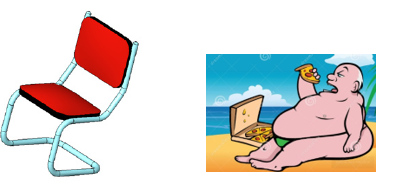
Figure 1: Imagine the person on the right to be sitting on the chair [1]. Will the chair endure? The first ten people who guess the correct answer will get free tickets to the island where the fat guy is enjoying the pizza.

In this case, if you intend to do an all-load-case FE analysis for the chair, you should consider nonlinear geometry.

Now, how small is “small displacement”? Can we quantify it? This is a question that needs to be answered with sound engineering judgment of the problem. Also, some thumb rules followed by FE analysts come to our rescue.

Thumb rule 1: If you are finding the deflection of a beam and the results show that the deflection is more than half of the beam thickness, then it is a must to consider geometric nonlinearity.

Thumb rule 2: Also check the strain in the model. If they are more than 5%, the geometric nonlinearity cannot be ignored.

Thumb rule 3: If the strain versus displacement relation is nonlinear, then consider geometric nonlinearity

Thumb rule 4: If the deformation is greater than 1/20^th of the component’s largest dimension, then consider geometric nonlinearity

But be aware that these are just thumb rules and not theorems that can be quoted. You will have to understand the problem, visualize how the results would be and then arrive at a judgment of considering or ignoring geometric nonlinearity.

Some examples:

Buckling is a good example of geometric nonlinearity.

To know more about linear and nonlinear buckling, check this informative article.

https://www.digitalengineering247.com/article/linear-and-nonlinear-buckling-in-fea/

Source: Wikipedia

Consider a simply supported beam. And a beam with both ends pinned. Now if there is a vertical load (perpendicular to the beam axis) acting on the beam’s midpoint, there will be no difference in the predicted displacement if geometric linearity is assumed and the forces are less.

If the load on the beam is increased significantly and geometric nonlinearity is considered, the vertical deformation in the two-end-fixed beam will be smaller compared to the simply supported beam. This is because there exists an axial force which reduces the vertical deformation in order to maintain the equilibrium.

To understand this phenomenon with a real-life example, visit this blog.

https://enterfea.com/geometrically-nonlinear-analysis-introduction/

I wish I had read this long time back.

The blog’s author has also made a flowchart (Figure 2) for deciding when to consider geometric nonlinearity.

Figure 2: Flowchart for deciding geometric nonlinearity [2]

Why do people use linear analysis then?

Can you give some more examples where one has to pay attention and consider geometric nonlinearity?

Are large deformation analysis and nonlinear geometric analysis, the same?

These are some questions I will answer in the Part 2

================================

Part 2

================================

It’s good that you now understand nonlinear geometry.

Do you know why geometric linearity has been used by CAE analysts for so long?

Some reasons are

• Analytical solutions are available for linear problems. This makes it easier for comparison or validation
• The linear FE models require lesser computational resources and are therefore very quick
• Standard analysis procedures dictate the need for geometric linearity
• Linear geometry assumption also facilitates a better conceptual understanding

Let’s move on to the next question?

When should you pay attention to the geometric nonlinearity?

If you think that the stiffness of the geometry changes due to the applied load.

It is difficult to quantify the shape change. I had given four different thumb rules in the previous article. Generally, commercial FEA software brochures have some guidelines. Some blog articles by FEA experts also have these.

Other than the shape change, you should also check how the direction of the load changes as the deformation progresses.

This is applicable especially in the case of large deformations and also depends on the commercial FE solver that you are using.

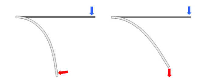
Figure 3: Follower load (left) and non-follower load (right) [1]

As can be seen from the above figure, the follower load changes its direction based on the deformation. Non-follower load doesn’t.

Now consider a pressure vessel subjected to very high pressure. This is bound to produce a shape change. And based on this shape change, the pressure load, which usually acts normal to the walls, needs to follow the deformation.

This in a way, takes us back to the thumb rules. Think carefully before you start the simulation. If you expect the deformations to be large, always consider geometric nonlinearity.

I had a misconception in nonlinear geometry. I used to think that stiffness does not change much when the deformation is small.

I found out, I was wrong after looking at this example where a flat membrane deflects under a pressure load as shown in the figure below.

Figure 4: Membrane under pressure load [1]

To quote from [3]

“Initially, the membrane resists the pressure load only with bending stiffness. After the pressure load has caused some curvature, the deformed membrane exhibits stiffness additional to the original bending stiffness (Figure 5). Deformation changes the membrane stiffness so that the deformed membrane is much stiffer than the flat membrane.”

Figure 5: Due to the deformation, it also acquires membrane stiffness. So linear geometric analysis underestimates the stiffness [1].

Concluding remarks:

Never jump into the CAE tool directly. First, understand the problem clearly. List out all the information that is provided and also the information you need. (Material properties, boundary conditions, etc.,). Then try to calmly visualize what the final result would be. I know this is difficult. But with some engineering sense and a rational mind, one can at least foresee the deformation trend based on the load case. This will save you a lot of time and hassles. And also help you in post-processing and report preparation.

Back to square one. Linear or nonlinear geometry? It depends.:) You will have to decide. Have a good time doing that.

Do you also have some interesting examples or experiences with geometric nonlinearity in FEA? Please do write about that in the comments section below. Would love to hear more and learn from you.

Have a great day.

Prost!

~ Renga

References:

[1] https://www.solidworks.com/sw/docs/Nonlinear_Analysis_2010_ENG_FINAL.pdf

[2] https://enterfea.com/nonlinear-flow-chart/

[3] https://www.solidworks.com/sw/docs/Nonlinear_Analysis_2010_ENG_FINAL.pdf

 

A book on Python Scripting for ABAQUS:

I have written a book that helps you to write Python scripts for ABAQUS in just 10 days.

Why should you buy my book?

Please use the link below to purchase the book.

Crash Course on Python Scripting for ABAQUS: Learn to write python scripts for ABAQUS in 10 days

Difference between h-method and p-method in FE Analysis (FEA)

There are basically two discretization approaches in FE analysis which are used to increase the solution accuracy as well as check for numerical convergence.

1. h-method

In this method, the number of elements is increased to have a finer mesh. The element type is not changed but only the number of the elements used for the analysis domain is increased.

“h” usually denotes the characteristic length of elements. This method is about reducing the “h” value which results in increased number of elements.

Figure 1: h-method [1]

If we look at the stress contours of a geometry which is approximated by a very coarse mesh (reduced number of elements), the stress distribution might deviate very much from the actual results and sometimes might also have stress jumps. This calls for a finer mesh as seen in the above picture.

2. p-method

This is the other method to increase the numerical convergence and move towards a more accurate solution. Here, the order of the shape functions is increased instead of increasing the number of elements. “p” denotes the polynomial order. By default, linear order shape functions are used by commercial FE programs. A quadratic shape function can have more accurate solutions.

Figure 2: p-method [1]

About the usage of p-element method from Altair University’s “Practical Finite Element Analysis” book

It has been documented in this book that the p-method is usually recommended for design engineers (CAD) who are in the initial design phase. At this point of the product design life cycle, they would not be too worried about carrying out a detailed analysis. Once the design engineers are satisfied with a basic feasibility analysis, they transfer the CAD data to the CAE team who in turn carry out the detailed and in-depth analysis.

So it is a god assumption to think in the lines of the p-method being used by the design (CAD) team in the initial phase and then the h-method being used by the analysis (CAE) team where detailed investigations and analysis need to be carried out.

And below is a snapshot [2] which complements the current discussion topic.

Prost!

~ Renga (Renganathan Sekar)

References:

[1] https://deust.wordpress.com/2014/11/30/h-method-p-method/

[2] http://innomet.ttu.ee/martin/MER0070/Loengud/FEA_Best_Practices.pdf

 

A book on Python Scripting for ABAQUS:

I have written a book that helps you to write Python scripts for ABAQUS in just 10 days.

Why should you buy my book?

Please use the link below to purchase the book.

Crash Course on Python Scripting for ABAQUS: Learn to write python scripts for ABAQUS in 10 days

Direct vs. iterative solvers in FEM

In FEM we usually solve for the equation [K]{u} = {f}

Here [K] is referred to as the stiffness matrix; {f} as the force vector and {u} as the set of unknowns.

The classification of solvers into direct and iterative mainly depends on the method of getting {u} in the linear equation. The selection of the solver depends on the process mechanics and problem size and is nowadays automatically chosen by most of the commercially available FE tools.

But as an engineer and analyst, it is good to know the back-end of what’s happening with respect to the solver selection. So here we go with a non-mathematical explanation of the differences between direct and iterative solvers used in FEM.

Direct Solver:

In the case of direct solver, you find the inverse of matrix [K] and then multiply with {f}. As this method involves inverting the matrix, it is mostly preferred for computationally less expensive problems. From literature, I understand that direct solvers are effective for problems with less than 100,000 unknowns. And the memory requirements are higher and the ability to solve the equations in parallel is difficult but not impossible.

Usually the direct solvers can be thought of as a variant of LU decomposition method where the [K] matrix is decomposed into a lower and upper triangular matrix (L and U respectively) in such a way that

[K] = [L][U]

More details about the method can be found here.

FE developers exploit the sparsity patterns in the stiffness matrix to increase the computational efficiency in the case of direct solvers by using established algorithms for solving sparse matrices.

What is a sparse matrix? – Read here.

Iterative Solver:

In the case of iterative solver, since finding inverse of a matrix is very time consuming if it is a very big matrix, they start with an initial solution(guess) and then gradually move towards the correct solution for {u}. Till a reasonably solution that satisfies the stop criterion (a tolerance value, usually) is obtained, the solver keeps iterating.

So, this is also not an exact solution but an educated guess. The search direction, i.e. the direction in which the initial guess moves towards the final solution is verified by using a variant of conjugate gradient method.

Iterative solvers are suitable for computationally big problems as they can often be parallelized more efficiently using algorithms. But there is a catch. For solving the linearized equations using the iterative solvers, your matrix needs to be properly conditioned.

“The art of devising a good iterative solver is to devise a good preconditioner!”.

–  Prof. Wolfgang Bangerth,

In the case of iterative solvers, sometimes oscillatory behavior might be observed. This means the initial solution does not move gradually towards the correct approximate solution and rather diverge. As an end user, you can find this by constantly checking the numerical output that is written by the solver. Unusually long computational times can also be a good indicator for this kind of a problem.

So how can you fix it?

Again, this method is something that has worked for me most of the time. My approach would be to check the model thoroughly if it is constrained properly. As in, try to fix the DOFs (DOF – Degree Of Freedom) in your analysis domain that might not have an impact on the simulation results. By doing this, you are reducing the potential errors gradually and assisting the solver converge fast.

And this is a very simplified and non-mathematical explanation of the topic which could be useful for a beginner or an application engineer who just wants to know which solver to use based on the problem context.

For a detailed and mathematical explanation, I would recommend going through this link. https://link.springer.com/chapter/10.1007%2F978-3-319-59038-7_5

Prost!

~ Renga

Other references:

[1] http://www.math.colostate.edu/~bangerth/videos/676/slides.34.pdf

 

A book on Python Scripting for ABAQUS:

I have written a book that helps you to write Python scripts for ABAQUS in just 10 days.

Why should you buy my book?

Please use the link below to purchase the book.

Crash Course on Python Scripting for ABAQUS: Learn to write python scripts for ABAQUS in 10 days

Difference between step, increment and iteration in a FE analysis

In the context of a FE analysis, I have often seen people getting confused with these terms – Step, increment and iteration – These terminologies can be conceptually confusing to a beginner. And the commercially available FE software use these terms in their own context making it even more complicated.

Photo by rawpixel on Unsplash

So, isn’t it good to know the definition of each of these terms and then know their purpose clearly? That’s the motivation for writing this article. Once you have a clear and a more generic understanding, it becomes easy to understand the results of your FE analysis irrespective of the FE tool that you are using.

Let’s get started.

Step

Any problem will usually consist of more than one step during simulation. Let’s assume that you want to simulate a simple contact analysis of a cylinder on a flat plate. So, this might consist of two “steps”. The first step would be to initially establish contact between the two entities and the second step would then be about applying the load.

The term “Step” broadly means the different steps in a process. This might consist of a loading step or a step where boundary conditions are applied.

Now you might think, hey what’s confusing here? Keep reading.

The confusion arises when the term “Step” is also used in the context of a solution step by some FE software. So, you have to be clear about the context where the term is used. Before I introduce what  a solution step means, I will write about “Increment” as they are almost the same.

Increment

In nonlinear FE analyses, the total load is usually not applied at once. This is rather split into a number of increments and then applied gradually. So “Increment” is the part of the total load that is applied gradually.

Now what happens after every “increment” depends on the type of solver – Implicit or Explicit.

In the case of an implicit analysis, an equilibrium is sought between the applied external force and the internal reaction force after every increment and accordingly the analysis results are recorded in the output database for post-processing. Implicit solvers are unconditionally stable. So usually the size of the increments is automatically decided by the FE tool.

To know the difference between implicit and explicit solvers with a practical example, check Difference between Implicit and Explicit FE analysis

The size of the increment is crucial in the case of an explicit solver. In order to have a numerically stable increment, the increment size must be below a stability limit and it mainly depends on the length of the smallest element.

Now that you know what an increment is, you can assume that a solution step is almost the same as that of an increment. To clarify with an example, if a load is applied in 1000 solution steps for a time period of 5 s, then the time step size or increment is 0.005 s.

Iteration

If you would have observed so far, we keep moving deeper after every definition. I mean, “Step” is the general and logical categorization of the problem at hand. “Increment ” in one step deeper and is a subset of a “Step”. And then comes “Iteration” where we go further into a “Step”.

As you know, in the case of an implicit solver, the equilibrium is sought after at every increment by checking the difference between externally applied force and internal reaction force.

This difference is called as residual (R).

Theoretically for equilibrium, R must be zero. As this is difficult, FE solvers usually have a tolerance value (a value close to zero) defined in their solver settings. Till the difference between the forces come under this tolerance value, the solver carries several “iterations”.

So, iterations are carried out within an increment in order to attain equilibrium. A solution is said to be converging if R value moves towards the tolerance value after every increment. The number of increments depend on the initial value as well as the robustness of the solution algorithm – for example Newton Raphson method.

I hope that you now have a general understanding about the different terms in a FE analysis.

Please do comment below if you have any questions.

Prost!

~ Renga

A book on Python Scripting for ABAQUS:

I have written a book that helps you to write Python scripts for ABAQUS in just 10 days.

Why should you buy my book?

Please use the link below to purchase the book.

Crash Course on Python Scripting for ABAQUS: Learn to write python scripts for ABAQUS in 10 days

Why should you buy my book – CRASH COURSE ON PYTHON SCRIPTING FOR ABAQUS?

7 reasons why you should buy my book: CRASH COURSE ON PYTHON SCRIPTING FOR ABAQUS?

1. Scarcity of comprehensive learning material

If you have already started/tried Python scripting for ABAQUS, you would have noticed the scarcity of step by step tutorial documents or guidelines. This book is a sincere attempt to address this concern by providing full python scripts for 9 problems from different categories with detailed comments.

2. Bypass the “starting trouble” like a boss

When it comes to learning a new skill, you might get confused due to a myriad of options. Some of the common pitfalls would be not choosing the right resources or not learning strategically. Add to this, the equally dangerous “starting troubles”. This phase is trickier and you have to cross this to accomplish your task. This book has been presented in such a way that the reader can effectively maneuver these inevitable pitfalls and actually start writing scripts that work.

3. Increase your productivity

Once you start following the practices in this book, I am sure that you can notice a significant increase in your productivity. Python scripts give you the leverage to automate repetitive tasks in FEM simulations using ABAQUS. Who doesn’t like to go home earlier?

4. Gain a better and practical understanding

Needless to say, by understanding and implementing efficient python scripting techniques for ABAQUS, eventually you will gain a practical perspective of the application of Finite Element Method (FEM).

5. Develop a problem-solving mentality 

When you practice this book’s techniques long enough, you will adopt a certain mentality while approaching newer problems which can be very helpful in solving them. These techniques can act as a mental framework to help you reduce trivial errors in FEM simulations and focus your energies on actual problem-solving.

6. Learn the skill in just 10 days

Time is precious. Period. I will directly jump into problems, emphasizing the solution methodology. My intention is to make you write efficient python scripts in ten days if you practice one chapter per day with this book. Of course, for a deeper understanding of FEM Theory or Python language, you will have to refer to standard textbooks.

7. Very affordable

You get this book at the cost of two coffees. Definitely a great deal right? My motive for writing this book is not money. I felt that I was writing Python scripts with ease and publishing my techniques in the form of a book with clearly explained examples would help people who are interested to learn the technique but have constraints in terms of money or time. This is the reason for pricing my book so low. But nonetheless, all the scripts have been tested many times and some parts of my scripts can be directly incorporated into yours to save time also.

If you would like the learn the technique for writing Python scripts for ABAQUS in just 10 days, please use the link below to buy the book.

Crash Course on Python Scripting for ABAQUS: Learn to write python scripts for ABAQUS in 10 days

Who will get the most out of my book – Crash Course on Python Scripting for ABAQUS: Learn to write python scripts for ABAQUS in 10 days

Beginners who are new to ABAQUS/Python scripting environment will find this book very valuable. I am sure that, as a beginner, if you follow the examples and practices in this book daily, you can easily start solving bigger problems from the industry with confidence, which is actually very important. Of course, you get refined by consistent practice and experience. But as clichéd it may sound if you have a strong foundation, it is comparatively easy to build on it. Compounding works great with knowledge too.

Academics can formulate their syllabus or coursework based on this book. As I have a Master’s degree in computational sciences from RWTH Aachen University, Germany and working currently in an academic-industry setting in South Korea, I am aware of the typical course structure in top universities for introductory courses based on the practical applications of FEM tools. I believe, the book’s contents and the order in which I have presented them can directly be used for coursework.

Graduate students who are working under tight deadlines to complete their thesis/internship will definitely find this book very useful. One of the important requirements from the perspective of your employer/supervisor would be the reusability of your FE methodology. It makes a lot of sense for them too as they can easily extend the scope of your work beyond your tenure. Using python scripting for ABAQUS can help you do that exactly with efficiency. And I do have a request for you, dear graduate students. I know the power of ‘word of mouth’. So if you found this book to be useful, please recommend this to your friends.

If you would like the learn the technique for writing Python scripts for ABAQUS in just 10 days, please use the link below to buy the book.

Crash Course on Python Scripting for ABAQUS: Learn to write python scripts for ABAQUS in 10 days

The ideal way to get the most out of my book:

The ideal way to get the most out of my book would be to follow the three suggestions given below.

1. I am a big believer of habits as consistent efforts are always very good and important in the long run. You will have to promise me that you will finish one chapter per day. This is a sensible target even if you are totally new to Python scripting.

2. You never have to memorize the syntax of statements or methods. ABAQUS Python scripting manual has detailed explanations for each and every command, its required and optional arguments. In this book, you will mainly learn the workflow of Python scripting, the methodology, and the process of writing scripts in general. It is always a good practice to have the scripting documentation by your side whenever you write scripts.

3. Of course, you can copy and paste the scripts directly from this book. I have tested them many times and it will work perfectly. But when you are trying to learn the art of scripting, please type them on your own and try making minor changes. You will definitely make some mistakes along this process which will reinforce your learning and make you even stronger.

A general tip:
If you are writing a script to automate a particular problem and get stuck up somewhere, try doing the same thing using the GUI and record what you do using a Macros in ABAQUS. After finishing the sequence of actions, you can have a look into the macros file which would be saved into your ABAQUS working directory. This file would be having the list of equivalent Python statements for the actions that you performed in the GUI.

Use the link below to buy the book.

Crash Course on Python Scripting for ABAQUS: Learn to write python scripts for ABAQUS in 10 days

Thank you so much.

~ Renga (Renganathan Sekar)

What is shear locking in FEM?

Sometimes, does your FE predictions of deformation end up lesser than the theoretical predictions?

Let’s see one of the main reasons why this happens – which is shear locking.

The unintentional generation of shearing deformation rather than the desired bending deformation is actually shear locking – Due to this the element becomes too stiff and the overall deflections are lesser.

This happens mainly with fully integrated linear elements subjected to bending loads.

This problem does not arise under normal or shear loads – occurs only during loads with bending.

In this post, I would like to explain the shear locking phenomenon with the help of an example from ABAQUS user manual.

If a structure is subject to pure bending moment M, the material distortion happens as shown in Figure 1.

Figure 1: Material deformation subjected to bending moment M

This of course happens in the actual material. If this is approximated by a linear element, then the edges of the curve cannot be represented. Figure 2 shows the deformation characteristics of such an element. The dotted lines are passing through the integration points.

Figure 2: Deformation of a linear element under bending

The lengths of upper and lower lines have changed indicating that they are under tensile and compressive loading respectively. But the important observation to be done here is the change in angle between horizontal and vertical lines. Before bending, it is 90°. Now this has changed. This is an indication that there exists some shear stress at these points. But theoretically, the shear stress of a material under pure bending must be zero.

Therefore, this shear stress is referred to as “spurious shear stress” and in FE literature, the usage of “spurious nodes” can also be observed frequently.

“Spurious shear stress” is induced because the curve is not represented by the element edges.

This means that the material shears instead of bending resulting in lesser deflection overall. This in turn causes the element to be stiff.

So how can this problem of shear locking be avoided?

By using higher order elements like quadratic elements which can represent the curve along the edges, the shear locking phenomenon can be avoided.

In general, it is a good practice to stay away from linear elements if there exists a bending load in your analysis.

In the next set of posts, I will write about full and reduced integration which will make the discussion in this topic more complete.

Please comment below if you have some questions on this post.

Prost!

~ Renga

A book on Python Scripting for ABAQUS:

I have written a book that helps you to write Python scripts for ABAQUS in just 10 days.

Why should you buy my book?

Please use the link below to purchase the book.

Crash Course on Python Scripting for ABAQUS: Learn to write python scripts for ABAQUS in 10 days

 

What is nonlinearity in FEM analysis? What are the different types of nonlinearities?

Almost all the applications that one tries to solve using FEM are nonlinear in nature. It is just that the FE analyst makes an engineering assumption avoiding the nonlinearity to make the computation simple. Provided, the FE predictions do not deviate much from the actual results because of this assumption.

So, what does nonlinearity mean in a FEM analysis? What are the different types?

Continue reading to know these answers.

Of course, from a perspective of structural mechanics simulations.

Generally, linear analysis means that the relationship between the applied force and the response to this force (Ex: displacement) is linear in nature. We know that this displacement can be obtained by inverting the stiffness matrix and then multiplying it with the force vectors. In other words, this means that the stiffness matrix does not change during a linear analysis.

If you want to have a quick recap of this methodology, have a look at this article

https://caendkoelsch.wordpress.com/2017/12/03/how-are-stiffness-matrices-assembled-in-fem/.

So now consider a situation where the stiffness keeps changing as the component deforms. Like for example, a forging simulation where the effective strain values at the end of simulation go up to 5.0 or even more.

This can be further emphasized by taking the example of a spring with linear and nonlinear characteristics.

As the stiffness is dependent on the displacement, which keeps changing, the initial stiffness matrix cannot be used without continually updating and inverting it during the course of the analysis. This is the reason why nonlinear analysis takes more time to solve compared to a linear FEM analysis.

Figure1: Linear and nonlinear spring characteristics (Source – Abaqus Manual)

Now let’s look into the different types of nonlinearity:

• Nonlinearity because of material behavior

This can be understood by referring to a stress strain curve (Figure 2). After point A in the curve, the stress versus strain relationship of the material is nonlinear. This is one sort of material nonlinearity based on the deformation or strain.

Now take the case of a hot forging process. Here the deformation is also dependent on other factors, for instance – temperature.

So this summarizes the first category of nonlinearity based on the material characteristics.

Figure 2: Stress strain curve

• Nonlinearity because of geometric conditions

Geometric nonlinearity arises when the changes in the model’s geometry are very high during the course of deformation. This happens when there are

1. Large deformations
2. Large rotations
3. Both
4. Initial loading conditions before the start of the analysis

• Nonlinearity because of boundary conditions

This situation arises when there is a change in the boundary conditions during the analysis. For example, consider the cantilever beam shown below. As the vertical deflection near the end of the beam increases and hits the stop, there is a change in the boundary condition.

All other contact problems fall under this category.

Figure3: Example for boundary conditions that change during the analysis (Source – Abaqus Manual)

I will end this article with some slides from the internet that I found useful regarding contact problems

Have a good day.

Prost!

~ Renga

Source: www2.mae.ufl.edu/nkim/INFEM/Chap5.pptx

A book on Python Scripting for ABAQUS:

I have written a book that helps you to write Python scripts for ABAQUS in just 10 days.

Why should you buy my book?

Please use the link below to purchase the book.

Crash Course on Python Scripting for ABAQUS: Learn to write python scripts for ABAQUS in 10 days